Ads Click Through Rate(CTR) Analysis And Prediction

Introduction to Ads Click-Through Rate Prediction:
Ads Click-Through Rate (CTR) prediction is a critical component of digital advertising. It revolves around predicting whether a user will interact with an ad by clicking on it. This prediction is based on various attributes and characteristics of the users and the ad content itself. By accurately predicting CTR, advertisers can optimize their campaigns, improve ROI, and allocate resources more effectively.
Dataset for Analysis:
For this project, we’ll be using a curated dataset containing relevant information about users and their interaction with ads. This dataset will serve as the foundation for training our machine learning model to predict click-through rates accurately.
If you wish to get an idea of how a production ready code should be like, check out the below code repository:
https://github.com/kshitijkutumbe/usa-visa-approval-prediction
Dataset link:
https://statso.io/wp-content/uploads/2023/01/ctr.zip
Now, let’s dive into the practical steps of performing Ads Click-Through Rate Prediction using Machine Learning in Python.
- we begin by making the necessary imports
import pandas as pd
import plotly.graph_objects as go
import plotly.express as px
import plotly.io as pio
import numpy as np

# sets the default background color to white for our visualisations.
pio.templates.default = 'plotly_white'- we then load our dataset
data = pd.read_csv('ad_10000records.csv')
data.head()
- time to define the necessary functions.
def EDA(df):
    """
    Performs basic Exploratory Data Analysis (EDA) on a DataFrame.

    Args:
        df (pd.DataFrame): The DataFrame to analyze.

    Returns:
        None
    """
    print("===== Shape =====")
    print(df.shape, end="\n\n")

    print('-'*80)

    print("===== Columns =====")
    print(df.columns, end="\n\n")

    print('-'*80)

    numerical_cols = df.select_dtypes(include=[np.number]).columns
    print("===== Numerical Columns =====")
    print(numerical_cols, end="\n\n")

    print('-'*80)

    categorical_cols = df.select_dtypes(include=['object', 'category']).columns
    print("===== Categorical Columns =====")
    print(categorical_cols, end="\n\n")

    print('-'*80)

    print("===== Info =====")
    print(df.info(), end="\n\n")

    print('-'*80)

    print("===== Description =====")
    print(df.describe(), end="\n\n")

    print('-'*80)

    print("===== Head =====")
    print(df.head(), end="\n\n")

    print('-'*80)

    print("===== Null values =====")
    print(df.isnull().sum(), end="\n\n")


def create_box_plot(data, x_col, color_col, title, color_map=None):
    """
    Creates and displays a box plot using Plotly Express.

    Args:
        data (pd.DataFrame): The DataFrame containing the data.
        x_col (str): The name of the column to use on the x-axis.
        color_col (str): The name of the column to use for color differentiation.
        title (str): The title of the plot.
        color_map (dict, optional): A dictionary mapping values to colors.

    Returns:
        None
    """
    fig = px.box(data,
                 x=x_col,
                 color=color_col,
                 title=title,
                 color_discrete_map=color_map)
    fig.update_traces(quartilemethod="exclusive")
    fig.show()

# Example usage:
# EDA(your_dataframe)
# create_box_plot(data, "Daily Time Spent on Site", "Clicked on Ad", "Click Through Rate based on Time Spent on Site", {'Yes': 'blue', 'No': 'red'})
By defining functions, you create blocks of code that can be reused in different parts of your project or even in other projects. This reduces redundancy and promotes code efficiency.
- time to examine our dataset.
# using our earlier defined function.

EDA(data)- Now let’s analyze the click-through rate based on the time spent by the users on the website
create_box_plot(data, "Daily Time Spent on Site", "Clicked on Ad", "Click Through Rate based on Time Spent on Site", {'Yes': 'blue', 'No': 'red'})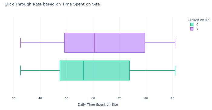
Based on the graph, it’s evident that users who spend more time on the website tend to click on ads more frequently. This suggests a positive correlation between time spent on the site and ad engagement. This insight can be valuable for targeting ad campaigns towards users who demonstrate longer engagement with the website, potentially leading to higher click-through rates. Now, let’s shift our focus to analyzing the click-through rate based on the daily internet usage of the users.
create_box_plot(data, "Daily Internet Usage", "Clicked on Ad", "Click Through Rate based on Daily Internet Usage", {'Yes': 'blue', 'No': 'red'})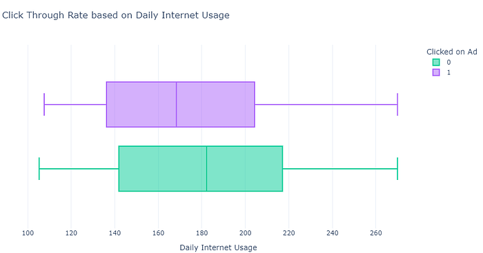
Based on the graph, it’s evident that users with high internet usage tend to click less on ads compared to users with low internet usage. This suggests that targeting ads towards users with lower internet usage might be more effective in terms of click-through rate. Now, let’s move on to analyze the click-through rate based on the age of the users.Now let’s analyze the click-through rate based on the time spent by the users on the website using the earlier defined function:
create_box_plot(data, "Age", "Clicked on Ad", "Click Through Rate based on Age", {'Yes': 'blue', 'No': 'red'})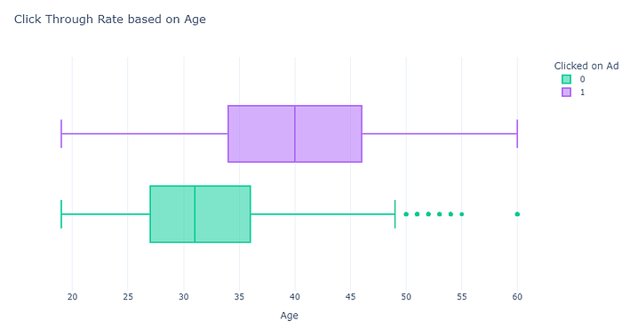
The analysis based on income provides valuable insights into user behavior. It indicates that users with higher age tend to click more on ads, suggesting a potential lucrative market segment. This information is vital for advertisers looking to optimize their campaigns and allocate resources effectively.
Now let’s analyze the click-through rate based on the income of the users:
create_box_plot(data, "Area Income", "Clicked on Ad", "Click Through Rate based on Income", {'1': 'blue', '0': 'red'})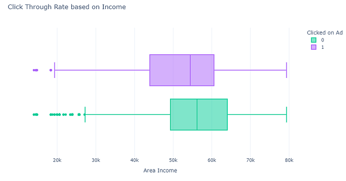
There’s not much difference, but people from high-income areas click less on ads
Now let’s calculate the overall Ads click-through rate. Here we need to calculate the ratio of users who clicked on the ad to users who left an impression on the ad. So let’s see the distribution of users:
# Calculate the total number of users who clicked on the ad
clicked_users = data[data['Clicked on Ad'] == 1]['Clicked on Ad'].count()

# Calculate the total number of users who left an impression on the ad
total_users = data['Clicked on Ad'].count()

# Calculate the overall Ads click-through rate
ctr = (clicked_users / total_users) * 100

print(f"Overall Ads Click-Through Rate: {ctr:.2f}%")
The interpretation of the click-through rate (CTR) depends on various factors, including the industry, target audience, and advertising goals. Here are some general guidelines for interpreting CTR:
High CTR: A high CTR indicates that a significant portion of users who saw the ad clicked on it. This is generally considered positive, as it suggests that the ad is relevant and engaging to the audience.
Average CTR: What constitutes an “average” CTR can vary widely depending on the platform, industry, and type of ad. In some industries, a CTR of 1–2% may be considered average, while in others, a CTR above 5% could be considered good.
Low CTR: A low CTR may suggest that the ad is not resonating with the target audience. It could be due to factors such as ad creative, targeting, or ad placement. However, it’s important to note that what is considered a “low” CTR can vary based on the context.
Context Matters: Comparing your CTR to industry benchmarks or previous campaigns can provide valuable context. For example, if your CTR is significantly lower than industry averages, it may indicate room for improvement.
Conversion Rate: While CTR is an important metric, it’s not the only one. Ultimately, the effectiveness of an ad campaign should also be evaluated based on the conversion rate (i.e., the percentage of users who take a desired action after clicking on the ad).
A/B Testing: Conducting A/B tests with different ad creatives, messaging, or targeting can help optimize CTR and overall campaign performance.
In summary, a “good” CTR is relative and should be assessed in the context of your specific goals and industry standards. It’s also important to track other relevant metrics and continuously optimize your ad campaigns for better performance.
Click Through Prediction Model.
- Now let’s move on to training a Machine Learning model to predict click-through rate. I’ll start by dividing the data into training and testing sets:
data["Gender"] = data["Gender"].map({"Male": 1,
                               "Female": 0})

x=data.iloc[:,0:7]
x=x.drop(['Ad Topic Line','City'],axis=1)
y=data.iloc[:,9]

from sklearn.model_selection import train_test_split
xtrain,xtest,ytrain,ytest=train_test_split(x,y,
                                           test_size=0.2,
random_state=4)- Now let’s train a random forecast classification algorithm:
from sklearn.ensemble import RandomForestClassifier
model = RandomForestClassifier()
model.fit(x, y)- Lets check the accuracy
from sklearn.metrics import accuracy_score, confusion_matrix, precision_score, recall_score, f1_score, roc_auc_score

# Evaluate the model
y_pred = model.predict(xtest)

accuracy = accuracy_score(ytest, y_pred)
conf_matrix = confusion_matrix(ytest, y_pred)
precision = precision_score(ytest, y_pred)
recall = recall_score(ytest, y_pred)
f1 = f1_score(ytest, y_pred)

y_prob = model.predict_proba(xtest)[:,1]
roc_auc = roc_auc_score(ytest, y_prob)

# Print the results
print(f"Accuracy: {accuracy:.4f}")
print("\nConfusion Matrix:")
print(conf_matrix)
print(f"\nPrecision: {precision:.4f}")
print(f"Recall: {recall:.4f}")
print(f"F1 Score: {f1:.4f}")
print(f"\nROC-AUC Score: {roc_auc:.4f}")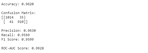
Conclusion
We performed an in-depth analysis of Ads Click-Through Rate (CTR) using Machine Learning. We explored the relationships between various user characteristics and their propensity to click on ads. Notably, we observed that users who spend more time on the website and those with lower daily internet usage tend to click on ads more frequently.
We trained a Random Forest Classifier to predict CTR based on these features. The model achieved a high accuracy, indicating its effectiveness in predicting user behavior.
Link to access the notebook on my github: